It’s 2024 and I haven’t updated this website in over 2 years so it’s time it gets some attention.
Click here to skip the preface-y section.
This is actually a project that I completed three years ago by following the Ray Tracing in One Weekend series while learning Rust. I originally implemented the ray tracer in C which got me caught up in a pointless search for micro-optimizations. I stopped after finishing reflections for metals. Then I tried implementing the same ray tracer in Rust which also turned into too much time spent on micro-optimization and not enough time spent on actually building the ray tracer.
If there was a lesson learned from that it would be to avoid doing something “for the sake of optimization” unless you actually looked at the emitted assembly. Compilers are crazy good these days. I don’t think I ever beat the compiler not counting algorithmic improvements. Sometimes even looking at the assembly isn’t enough because
- I’m not a seasoned assembly programmer
- There’s a lot going in the background during CPU execution that isn’t visible at the assembly level. Just because
gcc -O3employs some branchless code doesn’t mean the CPU will be executing your program faster (most of the times it will though).
So instead of trying to create the best ray tracer out there, why not try to create one using one of the slowest programming languages?
Python 🐍
I might write another article dedicated to explaining how Python works from source code to execution, but I’ll give a brief summary right now.
- Your source code is in a
.pyfile - You invoke the CPython interpreter with
pythonwhich will start reading your file - It goes line-by-line through your code and translates them into bytecode.
- It runs the simpler bytecode instructions (you may have noticed a
__pycache__folder when running code with module imports. Bytecode is cached there).
This process is unbearably slow since it has to do the translation process every single time it sees new code. Even if functions are already seen and translated to bytecode, the execution of the bytecode is still not native. This is contrasted with a programming language like Java which runs bytecode in the JVM which will run native machine code after translating the bytecode (JIT Compilation).
There are many attempts at speeding up Python like Numba package which JIT compiles your code without changes to the interpreter, or pypy which is an entirely separate interpreter that JIT compiles your code. I’ve used numba before and it can give on the order of 100x speedup.
Profiling Python code is one way to get a good idea of which parts of your code are slow and can benefit from these libraries. I used the cProfile program to get the timings.
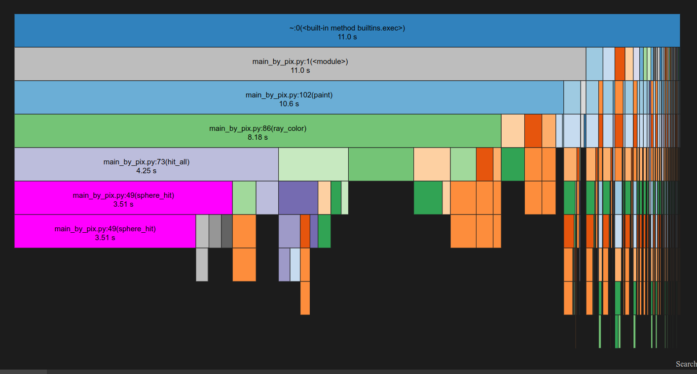 SnakeViz can visualize cProfile output.
NumPy is the best
NumPy isn’t recompiling your Python code to execute natively; rather, it’s already compiled to execute natively, and your Python code is the one calling it.
NumPy is a incredibly fast Python library implemented with C++. Manipulating large blocks of numbers (ndarrays or “Tensors”) tends to be a common theme in scientific computing and NumPy provides a convenient interface for a high level language like Python.
It’s still missing ample multicore support for common vector operations (e.g. all element-wise ops) but it does its best to run on multiple cores where it can if it’s linked against a good BLAS library.
All your program’s slowdown is now placed on CPython’s overhead. If you can keep it minimal then you’ve got code almost as fast as C++.
Ray Tracing in 30 minutes
If you draw a line from the origin (camera) to a pixel in a plane that is facing flat to the camera, you get a ray (a point and a direction).
All objects in a scene have a geometry and material. A ray might intersect with an object’s geometry (shape). If it does, then the material influence’s the hit location’s color and determines how the ray will scatter (choose a new direction).
Some general rules for materials
- Metals: Ray incident angle = Ray reflection angle. Good for mirrors
- Diffuse: Ray scattering is Lambertian. Pick a random direction to scatter the ray. Leads to smooth objects.
- Dialectric: Follows Snell’s law: \( \eta_1 \sin(\theta_1) = \eta_2 \sin(\theta_2) \). Materials that bend light like glass
Being able to tell if a ray intersects with an object depends on its geometry. The first Ray Tracing in One Weekend book only uses spheres.
This makes the math a lot simpler.
\[ \begin{align*} r^2 &= (x-c_x)^2 + (y-c_y)^2 + (z-c_z)^2 \quad (\text{sphere with radius } r \text{ shifted by c}) \\ &= (\vec{\mathbf{p}}(t) - \vec{\mathbf{c}}) \cdot (\vec{\mathbf{p}}(t) - \vec{\mathbf{c}}) \quad (\vec{\mathbf{p}}(t) \text{ is the ray}) \\ &= (\vec{\mathbf{p_0}} + t \vec{\mathbf{m}} - \vec{\mathbf{c}}) \cdot (\vec{\mathbf{p_0}} + t \vec{\mathbf{m}} - \vec{\mathbf{c}}) \quad (\text{expanding } \vec{\mathbf{p}}(t)) \\ &= \underbrace{(\vec{\mathbf{p_0}} - \vec{\mathbf{c}}) \cdot (\vec{\mathbf{p_0}} - \vec{\mathbf{c}})}_{c + r^2} + t \cdot\underbrace{ 2\vec{\mathbf{m}}\cdot(\vec{\mathbf{p_0}} - \vec{\mathbf{c}})}_b +t^2 \underbrace{\vec{\mathbf{m}}\cdot \vec{\mathbf{m}}}_a \\ \end{align*} \]
Subtracting \(r^2\) from both sides will give us \(a, b, c \) coefficients for solving the roots of a quadratic equation.
There are three cases:
- Negative discriminant (ray misses the object)
- Zero discriminant (ray skims the object)
- Positive discriminant (ray goes through the object, if it doesn’t bounce). Choose the \(t\) that gives the closest point.
The normal of the hit location, a vector perpendicular to the surface of the sphere, is computed by \( \overrightarrow{\mathbf{p_{hit}}} - \vec{\mathbf{c}} \).
The ray color is recursively computed: ray_color(old_ray_dir, world) = attenuation * ray_color(new_ray_dir, world).
In rasterization, the surface normal is dotted with the direction of the light source in the vertex shader to obtain shadows and lighting. In ray tracing, the normal is used for reflections.
Ray Marching
In this ray tracer, ray-to-object intersections are computed analytically. There is also ray marching which all the shadertoy demos use. Ray marching iteratively solves the hit location by using signed-distance fields of objects. The sphere equation used in this project is technically a signed distance field so switching to ray marching is not hard.
Path Tracing
Ray tracers capture reflections, but some objects in the scene may be dimly lit. It’s easy to achieve global illumination in an open scene where all rays don’t hit an object get assigned a bright color value but harder in enclosed spaces. There’s also some concern about the photorealism of ray tracing.
Ambient lighting is less pronounced in ray tracing because rays can only take paths from the camera. Those rays will also only get assigned a bright color value if they hit a light source. Another more general approach to ray tracing is Path Tracing: rays start from light sources and bounce their way to the camera. Path tracing produces better results but is slower since few rays cross the camera which is a single point so many rays need to be cast to sufficiently build an accurate color value for each pixel.
By The Book Python Implementation
Initially, I implemented the raytracer where all the steps of a ray’s bounces are computed one after another. Each ray’s color is computed independently, so there is some parallelism that can be advantageous.
Demonstration of what’s being done by a ray-by-ray (pixel-by-pixel) ray tracer shown here:
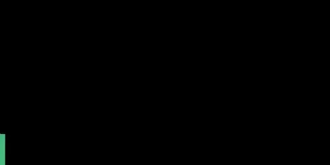 *not actually pixel by pixel* I just divided the work into blocks because the pixels are too small to see (it just looks like scan lines).
Multiple rays are actually created per pixel. The resulting color of all the rays in that pixel are averaged to create a smoother looking image. It’s not exactly the same ray that gets cast because the scattering for each ray may be random, but even if all scene objects were metals or transparent, each of these per-pixel rays have a slightly different initial direction. This also mitigates aliasing, a problem that is ubiquitous throughout science and engineering, especially in signal processing. An easy aliasing fix is to increase the sampling rate; in this case the sampling rate is the number of rays shot into a pixel.
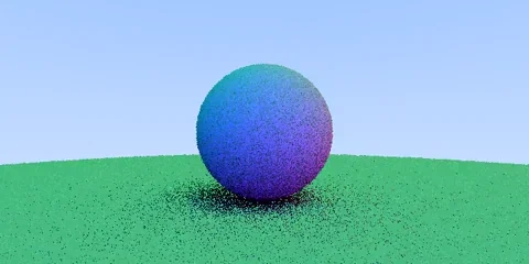 Increasing the samples per pixel. Can you see the difference?
Light Transport Equation
As an aside, this is also somewhat related to the Monte-Carlo method of computationally solving an intractable integral. In fact, the third book of the Ray Tracing series is dedicated to covering this. The color of each ray is determined by the Light Transport Equation (LTE):
\[ \text{Color}_o(\mathbf{\vec{x}}, \vec{\omega_o}, \lambda) = \int_{\vec{\omega_i}} A(\mathbf{\vec{x}}, \vec{\omega_i}, \vec{\omega_o}, \lambda) \cdot \text{pScatter}(\mathbf{\vec{x}}, \vec{\omega_i}, \vec{\omega_o}, \lambda) \cdot \text{Color}_i(\mathbf{\vec{x}}, \vec{\omega_i}, \lambda) \, d\omega \]
Taken directly from here. If path tracing had a Newton's second law, then this would be it.It says, “The color of an outgoing ray given its hit position and direction is the sum of the albedo multiplied by the color of the incoming ray, weighted by the probability that the ray scattered in that direction, for all possible ways to scatter. The wavelength, hitpoint, outgoing direction after scattering, and incoming direction influence the albedo color”.
Even though it’s a single integral, you actually have two degrees-of-freedom to sweep through if you really want to exhaustively compute it. Remember, this is a recursive function, so a single ray’s calculations grows exponentionally with bounce depth which is why Monte-Carlo is preferred.
The LTE is a very broad equation. In the context of this project’s ray tracer, \( \text{A}(…) \) is a constant depending on the material, \( \text{pScatter}(…) \) is always 1, and \( d\omega \) also equals 1… so there is no integral. When multiple rays are shot into the same pixel, it’s sort of like adding more sampling points (pScatter is the pdf we are trying to approximate, and multiple rays will choose to scatter in different directions) with equal probability.
Vectorizing
Ray Tracing in One Weekend implements Vec3 as classes and overloads the arithmetic operators. All scene objects are also classes that belong to a class heirarchy of hittable scene objects.
An immediate use case for NumPy is to replace Python Vec3 classes, but a complete render of a diffuse sphere still takes 640s. For reference, C and Rust take around 0.5s. There is still too much time being spent in CPython instead of actual computation due to overhead from control statements, stack management, indirection, etc.
Eliminating almost every loop
Instead of following a pixel-by-pixel execution order like:
build ray1, cast ray1, color ray1, build ray2, cast ray2, color ray2, build ray3, cast ray3, color ray3
It’s better to do stage-by-stage execution order like:
build ray1, build ray2, build ray3, cast ray1, cast ray2, cast ray3, color ray1, color ray2, color ray3
But if you vectorize one stage of the pipeline, then you need to vectorize all stages. The performance benefit is worth it though; the vectorized version runs in about 2s, 320x faster than the original. We let NumPy handle most of the computation, bonus points if it paralllizes anything (see np.dot), which will execute native instructions that can take advantage of architectural specifics dedicated to vector math like AVX.
Control flow by index masking
There are some parts of code that inevitably require control flow. For example, the discriminant must be checked before taking the square root. Luckily, the outcomes of these “fail” cases are usually “do not proceed” which means it is not included in the end result.
A negative discriminant means that there wasn’t a hit, so only take the positive values to move on to the next step (computing the square root).
But we also need to check if there’s two solutions. If there is, then take the hit point that is within a range of values.
This can be done by masking values to ignore those that cannot proceed. In practice, the indices of the values that satisfy the condition are used (whenever possible, below is an example where both are needed). I used timeit and a basic write-to-array example using indices and it completes 2.5x faster than with a boolean mask.
This is how it looks in code:
def is_hit_sphere(sphere_center: vec, sphere_radius: float, tmin: float, tmax: float, rays: np.ndarray) -> np.ndarray[bool]:
  # [ ... code that computes the a, b, c coefficients ... ]
  discriminant = b**2 - 4*a*c # these are element-wise ops
  has_hit = discriminant >= 0.
  sqrtd = np.sqrt(discriminant)

  valid_roots = np.ones_like(sqrtd, dtype=bool)
  roots = (-b - sqrtd) / (2 * a)
  # in sequential code, this would be if tmin <= root <= tmax
  first_roots_not_within_idx, = (tmin > roots | roots > tmax).nonzero() # use index

  # mask out a, b, c values instead of using the original ones to reduce computation of discriminant and its sqrt
  a, b, c = a[first_roots_not_within_idx], b[first_roots_not_within_idx], c[first_roots_not_within_idx]
  discriminant = b**2 + 4*a*c
  sqrtd = np.sqrt(discriminant)

  roots[first_roots_not_within_idx] = (-b + sqrtd) / (2 * a)
  second_roots_not_within_mask = tmin > roots | roots > tmax # *must* use mask

  valid_roots[second_roots_not_within_mask] = False
  has_hit[has_hit.nonzero()[0]] &= valid_roots

  return has_hit
Every frame starts with basically a 10 x 640 x 320 x 2 x 3 tensor and ends with a 10 x 640 x 320 x 3 tensor which is reduced to a 640 x 320 x 3 RGB image.
10 is the sample size, 640 x 320 the canvas dimensions, 2 x 3 for ray position and direction.
Over time, the rays will eventually get “culled”, whether it is hitting the scatter depth or not hitting anything. The has_hit value returned from is_hit_sphere(...) is a mask that can be used to select which rays get to live to the next depth of scattering. This is the biggest difference compared to the sequential, pixel-by-pixel ray tracer.
Some performance details: another difference is that the rays are not stored in a 3D, 4D, or any N-D structure really. It’s flat (treated like a list of 2D values, in the array-of-structures sense). This means that ray points and ray directions are right next to each other in the contiguous block of memory and loaded into the same cache line. Numpy does not actually move things around in memory when calling
.reshape()as it uses strided access so the colors can be reshaped to a 2D image at no cost. Putting cache aside, strided access could impact memory prefetching but the memory controllers these days are smart enough to detect strided access patterns. Finally, Ray Tracing in One Weekend uses a hit_record for every single ray but I use a structures-of-arrays pattern instead (writes to hit_records are indexed by the has_hit mask or indices).
Handling Materials
I could write the entire ray tracer without Python loop constructs if it weren’t for materials. Although I could still do it by either
- Cheating, using .map() over all scene objects
- Creating a
10 x 640 x 320 x 2 x 3tensor for every material
Neither are great options, so I stuck with a for loop over each scene object. Each scene object has an associated material id, so the type of material can be recorded in the hit_record. This is done by getting the indices / mask of rays that hit the object.
@dataclass
class HitRecord:
  # ... structure of 6 arrays ...
  material_idx: np.ndarray[int]

def hit_all(rays: np.ndarray, hit_records: HitRecord) -> np.ndarray[int]
  hits = np.zeros_like(rays, dtype=bool)
  for scene_obj, material_idx in all_scene_objects:
    obj_hits = is_hit_sphere(scene_obj, rays, ...)
    hits[obj_hits] = True
    # assign material to hit
    hit_records.material_idx[obj_hits] = material_idx

  return hits.nonzero()[0]
In Ray Tracing in One Weekend, each hit_record has a std::shared_ptr<Material> reference which uses the class type known at runtime to choose which scatter() function to call. I don’t use classes because there’s not point in packing extra data into the ndarray nor can I get any NumPy speedup with it. So the material_idx is the class type.
Instead of vtables, I do:
def ray_color(rays, scene_objects, depth, ...):
  # ...
  colors = # ... initialize
  hit_records = # ... initialize it
  hits_idx = hit_all(rays, hit_records)

  glass_idx, diffuse_idx, metal_idx, ... = get_material_arrays(hit_records.material_idx)

  new_rays = # intialize new rays
  new_rays[..., :, 0] = hit_records.hit_pos[hits_idx] # hit positions
  new_rays[glass_idx, :, 1] = scatter_glass(rays[glass_idx])
  new_rays[diffuse_idx, :, 1] = scatter_glass(rays[diffuse_idx])
  new_rays[metal_idx, :, 1] = scatter_glass(rays[metal_idx])
  # ... other scatter functions

  # this isn't correct code but a simplification since albedo needs to get multipled
  colors[hits_idx] = ray_color(new_rays, scene_objects, depth-1)
  # ...

  return colors
# fun fact:
A[[0, 1, 2], :, 2] = 81 # sets the array, but
A[[0, 1, 2]][:, 2] = 81 # does not
I could add a table of scatter functions to emulate the extra level of indirection of vtables, but there’s not point in doing that unless I have too many materials.
Color is tied to the material meaning new material ids must be created even if they have the same type of material. This isn’t necessary since you can always add another array to the HitRecords structure to store colors.
get_material_arrays is an interesting function because it gets slow if the number of materials exceeds log(num_rays). It’s possible to do an argsort() to get the material arrays, but the simplest solution is
def get_material_arrays(material_indices):
  all_material_indices = []

  for k in range(MAX_MATERIAL_IDS):
    all_material_indices.append((material_indices == k).nonzero()[0])

  return all_material_indices
Random Unit Vectors
Getting random vectors is a critical section, both in the threading sense (contention over RNG) and the performance sense (called by every scatter function), of the code. It’s not correct to randomly pick \( \theta \) and \( \phi \) to get points on a sphere for the same reason why you can’t for a circle.
The function I have is very inefficient (batched pick and reject), so there’s room for improvement.
Einsum
I used einsum() in one other project (gradient of vector w.r.t to matrix) so I’m new to this function.
The best way to think about it is to think that you are summing over all the indices missing on the right hand once you take the dot product of the ones on the left.
np.einsum('ij, ij -> i', A, B)
I had to use it because np.dot() can’t “take dot product between each vector in two list-of-vectors” without a for loop.
Ray Tracing in TensorFlow or PyTorch
PyTorch and TensorFlow are both libraries for computation graphs, automatic differentiation, and tensor manipulation. They are highly optimized for computing the gradients of a function. I will dedicate an article in the future to explaining them.
It’s pretty easy to port the code to PyTorch. Just need to
- Replace all instances of
np.ndarraywithtorch.Tensor - set default device to GPU and add
.to(gpu_device)where needed - Be careful with
tensor[indices, :, 1]which might give slices oflen(indices) x 1 x 3instead oflen(indices) x 3 np.random.uniform(shape)->torch.FloatTensor(shape).uniform_()np.fabs->torch.abs()np.isclose(arr, 0., atol=1e-8)->(torch.abs(arr) < 1e-8).all()(torch has.isclose()but does not broadcast the comparison)
For some reason, even though PyTorch enables multithreaded einsum(), the code is still 8x slower than the NumPy.
Wrapping up
Vectorized code is easily parallelized, but I don’t directly leverage any kind of core-level parallelism. Rendering still takes a while even if each frame takes 5s.
There are libraries that enable multicore parallelism, but it was easiest for me to just assign each thread a range of frames to work on given the same code.
Here’s the final result. It took 20 minutes to complete which is way slower than the path tracers that can even run in the web browser.
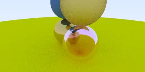 Blue diffuse sphere, yellow diffuse sphere, yellow metallic sphere, and red dialectric sphere