Is it possible to determine the best fitting curve to a series of data points just by knowing the form of the function?

The Perceptron

The perceptron, a perceptively simple unit of the neural network, can demonstrate powerful predictive performance when given the right data.

The most basic task that everyone’s heard of is binary classification. Perceptrons a great at solving these problems because if they are presented data with a definite boundary separating the two classes of data, then they can predict where unseen data points may lie.

There main limitation of this current perceptron model is its ability to only separate data points that are “linearly separable”. If the number of columns in the data is 2, then the points are separated by a line. Three, then separated by a plane. Four, then a hyperplane… and so on.

With a few tweaks, one will be able to get the perceptron to do tasks like non linear regression. But first, let’s take a look at the special case of linear regression.

The Linear Regression Problem

Every line represented by a function is in the form y = ax + b. Given a bunch of linearly separable data (data pints that could be separated by a line), could you find the line drawn by a and b?

As a normal human being, I would say, “Sure, I’ll just draw something like this”

My hand drawn line

You’re able to tell what the line is because of the grouping of the points and the overall trend, but how would a computer be able to tell this though? Let’s begin by critiquing the computer.

The Cost Function

*It's basically the same as the loss function. You will hear them being used interchangeably*

Let our current model (our best guess) be a function of a and b: f(x) = ax+b and given a set of points in the form of (x, y), and the i’th point is (x_i, y_i), we can apply the sum of square errors to find the cost C(a, b) = sum((y_i-f(x_i, a, b))**2).

We want to be minimizing the error (the cost) by finding the best values of a and b, but we don’t know what to do. We could try guessing the parameters… or even try all of them (grid searching), but that will take too long!

Using knowledge from multivariable calculus, you could try holding x fixed and then treating C(a, b) as a surface– then maximize using the second derivative test. This is known as the analytical way of achieving the optimum a and b and it’s guaranteed to work all the time.

The catch is that it doesn’t work on a broader class of nonlinear regression problems.

The Perceptron Approach

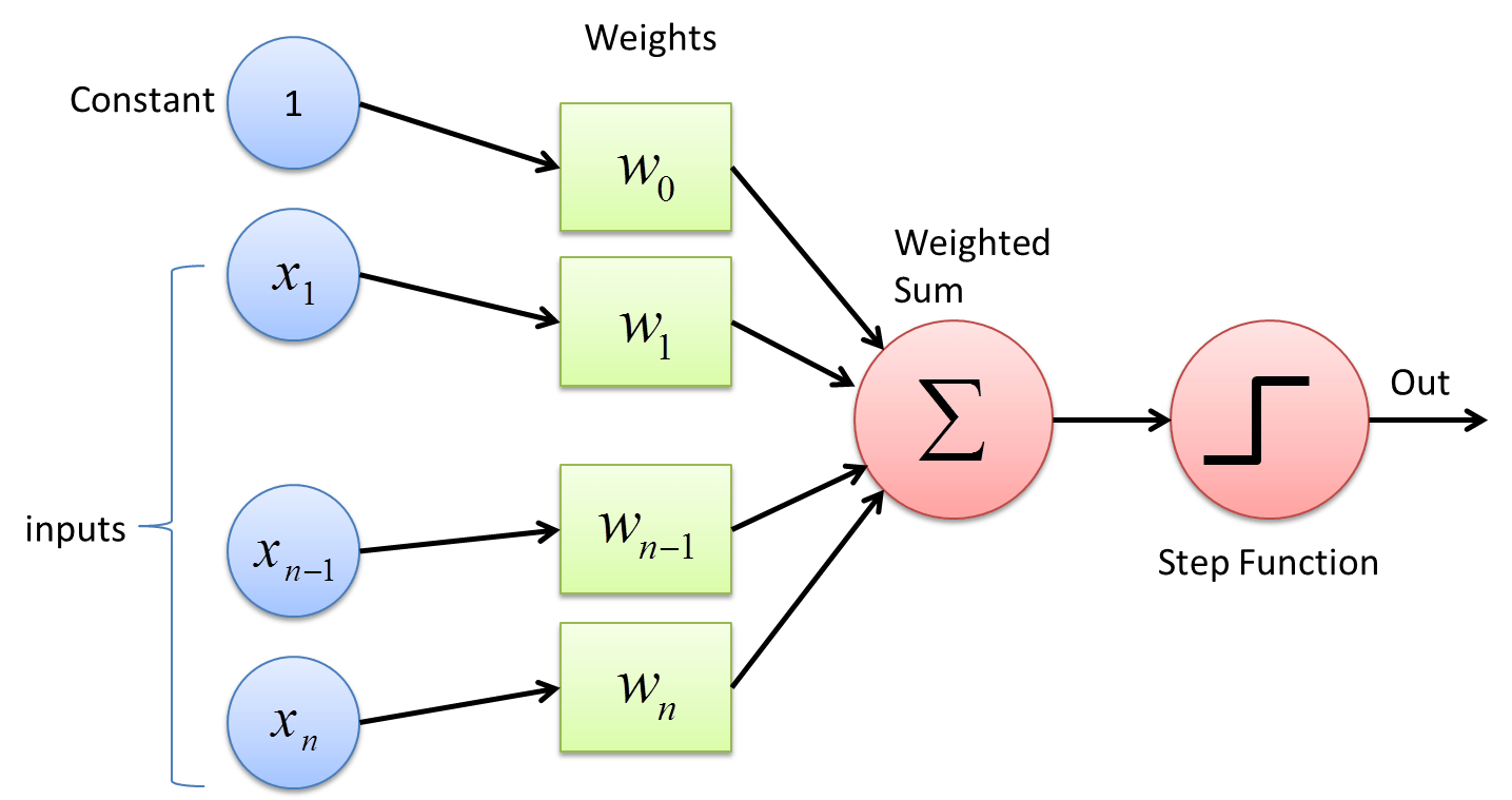The Perceptron

A perceptron has a number of inputs, a number of weights, and a step function. The inputs and weights are vectors and the activation function function works on scalers. Taking the dot product between the inputs and weights is the net input and the net input is passed through the activation function, which is sometimes just the net input itself (linear activation).

This works well in modeling our linear regression problem because all of the inputs are multiplied by some parameters that we’re trying to optimize. In this case, b can be represented by the bias of a perceptron (a value that always adds to the net input to prevent the perceptron from fitting too closely to the input data). The bias normally serves another purpose but it’s a convenience here to represent the constant b as it sits without an input.

We can then calculate the cost using the cost function described earlier.

Gradient Descent

The weights of the perceptron are initialized to small but random values at the start of the perceptron’s life. Sticking with our surface analogy, let’s visualize our network’s weight ‘surface’.

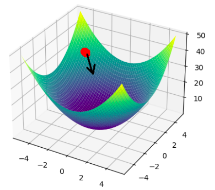The Weight Surface.

Gradient descent tells us that to minimize our parameters, we need to take the steepest path from our current position. The common analogy is a ball rolling down a rough hill.

You can find the steepest path by taking the negative of the gradient (partial derivative with respect to each weight) of the cost function. We have to then step by a very small amount to adapt to the roughness of the weight ‘surface’ by the “learning rate” hyperparameter.

import numpy as np
import matplotlib.pyplot as plt

fuzz = np.random.normal(size=(200), scale=50)
x = np.linspace(0, 100, 200)
y = 5*x+10+fuzz
w = np.random.normal(size=(2), scale=0.1)
for _ in range(15000):
    err = sum((y-(w[1]*x+w[0]))**2)/len(x)
    d_err = sum((y-(w[1]*x+w[0]+0.0001))**2)/len(x), sum((y-((w[1]+0.0001)*x+w[0]))**2)/len(x)
    gradient = (d_err-err)/0.0001
    w += -0.0002*gradient

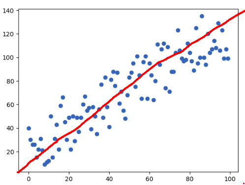
plt.scatter(x, y)
plt.plot(x, w[1]*x+w[0], color="lime")
plt.show()

Polynomial Regression

So what if we have a polynomial model that we need to fit to data? The process doesn’t change.

We can start with constructing the hessian matrix (to find the minimum of the surface– even though it’s not a surface when there’s more than 2 weights) and then taking its determinant. There’s a lot of symmetry involved and lots of things should cancel out giving you the coefficients of the polynomial fit.

Nonlinear fitting

Borrowing the concepts from above, we could use this property of gradient descent and cost minimization to find the appropriate weights that match a function’s description.

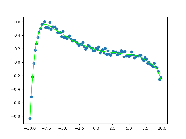
For example, if I had the some scatter plot data and a model function sin(ax+b), I can choose a and b to be the weights of the perceptron, and be able to find the cost value to be used to tweak the a and b values.

Here is an example of a very tight fit between the network’s weights plotted against scattered data fed into a function with similar weights with random noise added onto it.

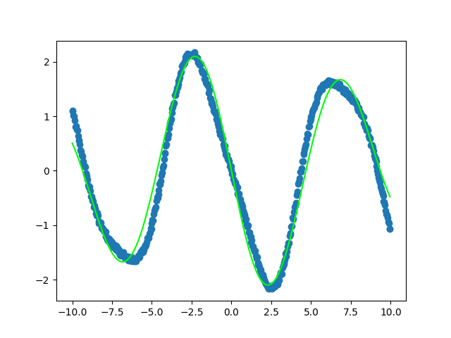The tight fit

Conclusion

I stopped working on this blog post for a while and picked it back up months later. Lots of details were lost along the way so the post is written incohesively.

Here is the link to the source